Documentation for CAP6400's Midterm & Final Project
2004-12-01
| Revision History | |
|---|---|
| Revision 2.0 | 2004-12-01 |
| Release for Final Documention: Added Chinese Number Detection | |
| Revision 1.0 | 2004-10-16 |
| First Release for Midterm Documention. | |
Abstract
An implementation of a tool/tutorial for basic image processing algorithms. The type of algorithms include point and neighborhood operations. This document doubles as a basic user manual for non-technical users and a tech manual for the tech-savvy user.
Table of Contents
- 1. GUI Layout
- 2. Basic Usage
- 3. Technical Guide
- 3.1. Windows API
- 3.2. OpenGL
- 3.3. Mathematics and Algorithms
- 3.3.1. Gray-scale Conversion
- 3.3.2. Pixel Complementation
- 3.3.3. Adding Constant to Pixel
- 3.3.4. Adding Percentage to Pixel
- 3.3.5. Random Noise
- 3.3.6. Averaging Neighborhood
- 3.3.7. Median Neighborhood
- 3.3.8. Edge Detection
- 3.3.9. Distance Map
- 3.3.10. Histogram Equalization
- 3.3.11. Histogram Scaling
- 3.3.12. Adaptive Histogram Equalization
- 3.4. Chinese Number Detection -- Algorithms
An overview on the graphical user interface layout of IMGPROC.
There are four windows that make up IMGPROC:
The Main Window: Where images are brought into the program and displayed. Also, where operations are applied to those images.
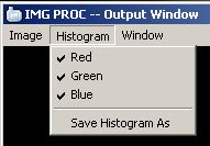
The Main Window's Histogram: Where the relative histogram of the main window's image is displayed
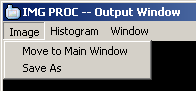
The Output Window: Where the output image of an operation from the main window is displayed
The Output Window's Histogram: Where the relative histogram of the output window's image is displayed
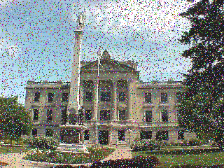
Both the main window and the output window can save their currently displayed image to disk. They can also save the histogram of the currently displayed image to disk. A screen shot of the program running:
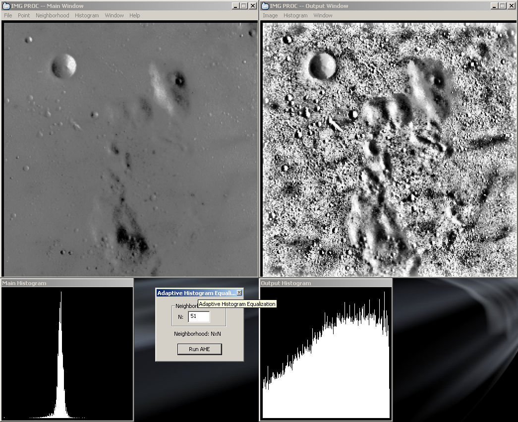
IMGPROC: Inaction as a whole
The main and output windows both have menus, the histogram windows do not. The output window's menu is minimal, consisting of items for saving, moving, clearing, and histogram color viewing only. The main window's menu has the same abilities plus all the image manipulation operations provided by IMGPROC.
This section goes through each menu item in the main window.
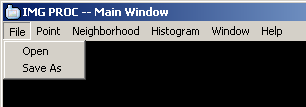
File -- used for opening and saving image files. Possible formats are PNG, PPM, and PGM.
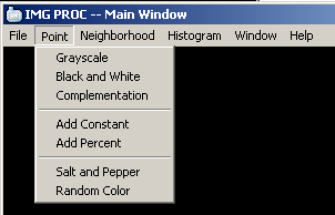
Point -- point operations on a image
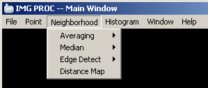
Neighborhood -- neighborhood operations on a image
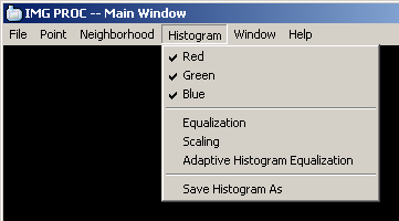
Histogram -- histogram operations and options
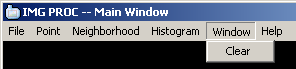
Window -- contains operation to clear the window
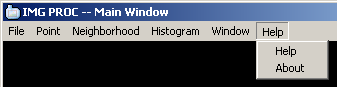
Help -- tell about IMGPROC and links to this document
This section is intended for non-computer science majors while still acting as a quick overview of operations for the tech-savvy.
Pixel -- Two forms: RGB(color) and gray-scale
RGB -- Component colors Red Green Blue, each have a value [0,255], all 0's is black, all 255's is white
Gray-scale -- One component describing a shade of gray, value range [0,255], 256 possible gray shades
Neighborhood -- A matrix, usually NxN, made up of pixels values that surround a center pixel value in question
Mask -- A matrix, usually NxN, made up of numeric values used in mathematical operations on neighborhoods
Point operations are manipulations on each pixel without any information about its neighboring pixels
Converts each color pixel into its gray-scale representation
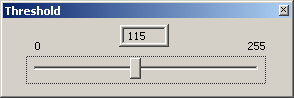
Converts each pixel to either black or white depending on a threshold. If the pixels gray value is less than the threshold it becomes black, else it becomes white. The threshold parameter is adjusted with a slider control dialog, below:
Reverses the pixel values, black becomes white, white become black and so on throughout the whole color range.
 |  |
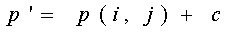
Add a constant value to every pixel, value range [-255,255]. A positive value brightens the image, a negative value darkens the image. The constant value is adjusted with a slider control dialog.
Add a percentage to every pixel based the pixel itself, value range [-255%,255%]. This operation helps bring out the contrasting colors. A slider control dialog adjusts the percentage.
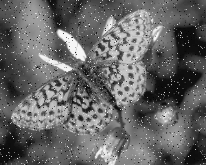
Adds in black and white pixels in random locations of the image. The number of random pixels inserted is a percentage of the total amount of pixels in the image. The percentage is control by a slider dialog.
These operations use neighborhoods and masks to manipulate images. Every operation on a pixel needs to have knowledge of neighboring pixels.
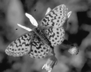
This operation reduced noise. A neighborhood, 3x3 or 5x5, of the current pixel is constructed with the center pixel being the pixel in question. All the pixel values are average and that average is the new pixel value. Gray-scale images only.
This operation reduced noise. A neighborhood, 3x3 or 5x5, of the current pixel is constructed with the center pixel being the pixel in question. The pixels are sorted and the middle value is the new pixel. This is a better noise reduction operation then averaging. Gray-scale images only.
3x3 Median Filter:
 |  |
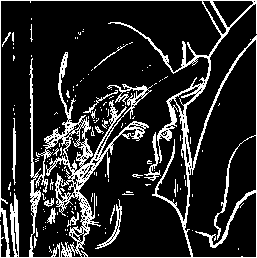
Edge detection is used to define edges within a image. This could be a door way or even shadow. Many have come up with their own operators for defining an edge, IMGPROC uses two of them plus the ability to define your own mask(advanced users). Sobel 3x3 and Laplacian 3x3 are the two operators provided.
A threshold slider control dialog will appear when edge detection is selected. Using it will add or decrease the amount of edges found in the image. Edge Detection is only from gray-scale images.
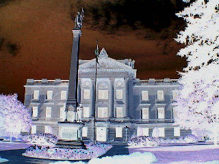
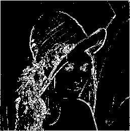
Nice for giving a cool effect to edges. Gradient areas of an image are places where color is changing over a distance.
 | 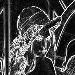 |
An example of Sobel's operation
|  |
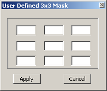
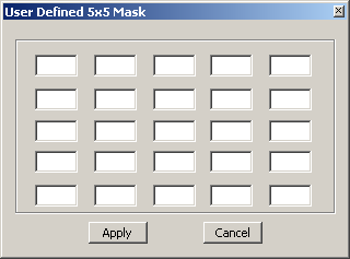
Define your own 3x3 Matrix to detect edges.
A distance map of an object depicts the distance from the edge of the object in gray-scale color. The further a pixel's distance is from the object's boarder the brighter the pixel gets. This can be used to define a skeleton of an object. For IMGPROC, objects are white and background is black.
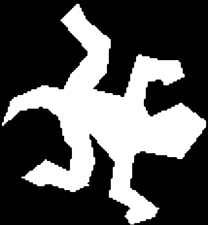 | 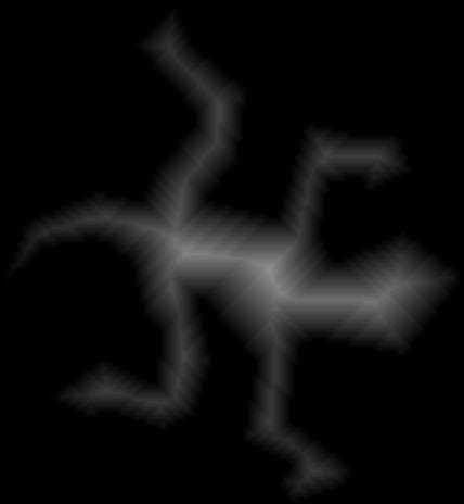 |
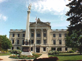
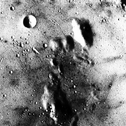
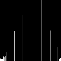
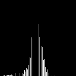
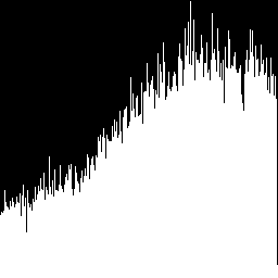
The histogram of an image is the graph of the different frequencies of color values. The x-axis is the color range [0,255] and the y-axis is the frequency of those values. The y-axis is scaled to fit the window properly. An example of an image and its histogram below:
 |  |
These check menus toggle the colored histograms. If red is not checked, only the green and blue histograms show, etc. Has no effect on gray-scale image histograms.
This operation is an attempt to flatten the histogram by uniformly distributing the pixels values over the gray-scale range.
 |  |
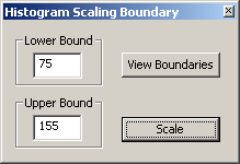
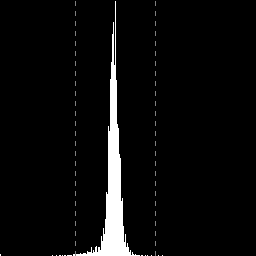
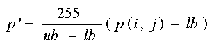
A stretch of the histogram is conducted with this operation. A lower and upper bound is defined. Anything below the lower bound becomes black. Anything above the upper bound becomes white. Anything between the boundaries is stretch over the gray-scale range.
A dialog window is used to define the bounds. The view boundaries button will draw dotted lines on the histogram where the bounds exist. The scale button will run the operation, below:
 |  |
Final Result:
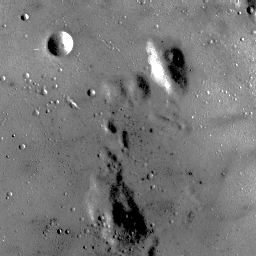 |  |
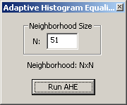
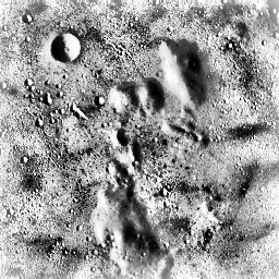
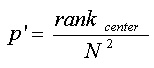
This operation can bring out details not usually since in a image. Used in medical image processing. Gray-scale images only. AHE uses a dialog window to define the square size of the neighborhood. N must be between 3 and 101 and ODD.
AHE Result:
 |  |
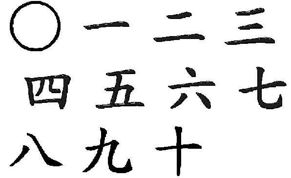
This function of IMGPROC is used to detect a single black chinese numeral on a white background. The possible numerals that can be detected are 0 thru 10. Once this function is selected the analysis will begin and when finished a message box will appear with an answer. This answer can be one of three types. The first can be correct match (hopefully) giving the arabic numeral the chinese numeral represents. A second type can be a group of numbers that IMGPROC thinks are possible the correct answer but is not sure which one in the group is the actual answer. The last answer type is "no match". The chinese numerals that IMGPROC can recognize are below. The algorithms used by this function can be found in the Technical Guide of this document.
This section is for the tech-savvy. Algorithms, math, and structures will be discussed
IMGPROC was built with the Windows32 API, more information on the WIN32 API can be found at msdn.microsoft.com.
A good book for learning the WIN32 API basics can be found at amazon.com.
IMGPROC uses OpenGL to display images, taking advantage of its double-buffer capabilities. More information on OpenGL can be found at opengl.org. IMGPROC does not use OpenGL to manipulate images, the only important function from its library that is used, is glDrawPixels:
glDrawPixels(image->width,image->height,GL_RGB,GL_UNSIGNED_BYTE,image->rgb_bpixels);
glDrawPixels(image->width,image->height,GL_LUMINANCE,GL_UNSIGNED_BYTE,image->gs_bpixels);
The first call is for RGB images, the second is for gray-scale images.
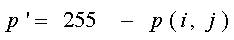
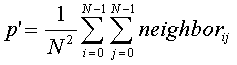
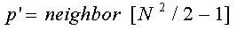
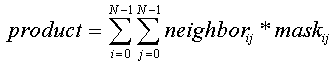
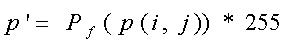
Images are defined at a 2D array of bytes. p(i,j) is the color value at location i, j. p' is the new color value for the current i,j.


If bool is false, change current pixel to random noise. c is the percentage of noise desired.
If N = 3, then the neighborhood is 3x3 with the center at (1,1).
If product is greater then Threshold, current pixel become white, else it become black.
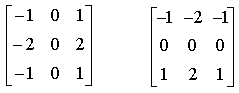
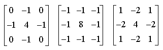
A 3x3 mask filled with 1's is used to erode an object. The mask is applied across the image, if the mask matches the current neighborhood then the center pixel of the neighbor is stay in the image. If the mask doesn't match the mask the pixel is marked for deletion. After every pixel in the image is examined, the pixels that are marked for deletion are deleted. Next, a counter that represents the number of erosion's preformed thus far is incremented. The whole operation is restarted and continues till there are 0 pixels marked for deletion. At this point the object in the image will be delete from all the erosion operation.
When a pixel is deleted, it get a new value which is based on the number of erosion's that had happened up to this point. Pixel values moving toward the center become brighter since more erosion's have taken place to reach those pixels.
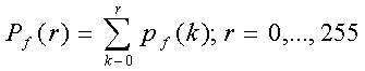
W is the image width, H is the height. Hf(k) give the frequency of color value k in the image, so k is in the range [0,255]
Steps Involved
Binary Conversion using a threshold of 50. This removed any artifacts from the scanning process.
Closure Morphology was used in a attempt to get rid of holes within the numeral. The operation was performed with a 3x3 mask filled with zeros representing black. Two dilations were performed followed by two erosions. A dilation operation works by taking a pixel's 3x3 neighborhood and comparing it with the 3x3 mask, if at least one neighbor is black, then the current pixel become black. An erosion operation is the same but ALL neighbors must be black to change the current pixel to black.
Horizontal and Vertical Line Counting was used to figure out how many horizontal and vertical lines made up the chinese numeral. Pixel histograms were constructed with larger peaks representing a line. The technique for horizontal line counting will be discussed only, the vertical technique is symmeteric.
The first step was to construct the pixel histogram, this is different from an image histogram made up of color values. The pixel histogram represents the number of pixels on a horizontal scan line. This is simple, the x-axis of the histogram is the height of the image. The ith horizontal line is scanned, counting the number of black pixels then assigning that value to the ith x-axis value of the histogram. Once at the bottom the histogram is complete. Next, a 5x5 median filter and closure was applied to the histogram to get rid of very small hills and valleys. Last, a line scan from top to bottom was performed on the histogram to find the number of peaks. The line gave the number of intersection it ran through. The scan did not stop until the current number of intersections was less then the max intersection seen thus far. A rule was thrown in to ignore peaks of height five or less. The number of lines returned was the (last max)/2.
The vertical and horizontal line histograms are output in pgm format to the directory from which the chinese numeral was read.
Thinning was used in preparation for finding feature points. The Zhang-Suen thinning algorithm was used for this operation. To learn how the algorithm works read my presentation on Skeletonization pages 26 - 29. Staircase elimination was used for skeleton cleanup, Holt's method can also be found in my presentation page 33. Sometimes the thinning algorithm would connect close objects that where not connected in the orignal image so a ditial substraction of sorts was conducted to eliminated that drawback. A pixel in the skeleton was removed if that same pixel in the orignal image didn't exist.
Feature Point Detection was used on the skeleton. Feature points of use for this project were end-points, 3-ways intersections, and 4-way intersections. Coordinates within the image for each on the feature points were recorded. A skeleton pixel with only one neighbor was recorded as an end-point. A skeleton pixel with connectivity of 3 was recorded as a 3-ways intersection. A 4-ways intersection was record to be a skeleton pixel with connectivity of 4. To learn more about connectivity read my presentation on skeletonization.
Corner feature points were not detected :(
Feature Point Reconciliation is an operation used to even out the playing field for different sized chinese numerals. First, all feature points were scaled to a constant size. Therefore eliminating the size issue. Next, feature points were combined under specific rules since the thinning algorithm did not produce perfectly straight lines. One 3-way intersection within a threshold(very small) distance of 2 or more end-points were combined all into one end-point. Two 3-way intersections within a threshold distance of each other were combined into one 4-way intersection. An end-point within thresholds distance to a 3-way intersection were both eliminated. Last, two end-points within a thresholds distance and no pixels in between them were emliminted. The last two rules are elimination rules because they both produce corner points which IMGPROC does not take into account at this time (version 3...).
Answer Phase was conducted as a primary and secondary lookup table. The primary table consisted of just feature points. Each number could have more than one feature point set. Once primary table lookup was complete, secondary table lookup began if more then one match was found in the primary table. The secondary table holds two elements, number of horizontal lines and number of vertical lines, with the possibility of having more then one entry for a number.